Barnes-Hut Algorithm for N-bodies Simulations

drag rotatescroll zoomWASDrotateR / F zoom

Interactive 3D Octree structure for auto-gravitational system.

Introduction

I still remember the day I discovered numerical integration in my numerical physics course, it felt like a bright, almost magical moment. I suddenly realized that I finally could take my revenge of first-year physics student trying to solve the three-body problem (not knowing it has no general solution)... I went straight to my computer and coded a small simulation ! The dance of those three spinning planets was printing stars on my eyes ! Three planets ! Then the Solar System ! Why not the whole galaxy !? I was incredibly enthusiastic but so naive... I broke my teeths on the brutal tyranny of $O(N^2)$ .

A few years later, I discovered the Barnes–Hut algorithm, and finally, I defeated the tyranny... Here is how to do it :

The N-body Problem

The $N$ -body problem is a classical mechanics system in which $N$ bodies interact through a given force. I'm going to have the audacity to remind you briefly how this works...

The dynamics of the system obey Newton's second law: the acceleration of each body depends on the force applied to it,

m_i \vec{a}_i(t) = \vec{F}_i

In the case of a gravitational system, the force acting on body $i$ depends on the positions of all the other bodies:

\vec{F}_i = \sum_{j \neq i}^N \frac{G m_i m_j}{||\vec{x}_i - \vec{x}_j||^2+\epsilon^2}\vec{u}_{ij}

Here, $\vec{u}_{ij}$ is the unitary vector going from $\vec{x}_i$ to $\vec{x}_j$ , $G$ is the gravitational constant, and $\epsilon$ is a softening (regularization) parameter introduced to avoid numerical divergences when bodies get very close to each other.

Once the forces are computed, we can integrate the system in time. An efficient (and underestimate !) choice is the Verlet integrator:

\vec{x}(t+\Delta t) = 2 \vec{x}(t) - \vec{x}(t-\Delta t) + \vec{a}(t)\,\Delta t^2 + \mathcal{O}(\Delta t^4)

In principle, this allows us to compute the positions of all bodies at the next time step.

However, the computational cost of evaluating the forces quickly becomes prohibitive as $N$ increases. Indeed, the naive approach requires computing all pairwise interactions, leading to a complexity of $O(N^2)$ , which becomes the major bottleneck for large systems.

Barnes–Hut Algorithm

This is where our friends Barnes and Hut come to the rescue (if they are indeed real people, to check...). The algorithm that took their name allows us, with a slightly more complicated implementation, to reduce the computational complexity to $O(N \log N)$ .

The key idea is to exploit the fact that gravitational forces decrease with distance. Far-away groups of bodies can be approximated as a single "virtual" body, reducing the number of interactions that need to be computed.

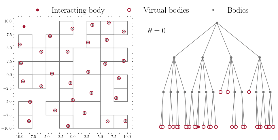
The algorithm works by building an octree structure: space is recursively subdivided, and bodies are organized hierarchically according to their positions. Groups of distant particles are then approximated by virtual quantities (virtual mass and center of mass).

Everything is controlled by a hyperparameter $\theta$ . At each time step, the algorithm proceeds as follows:

Construct the Tree

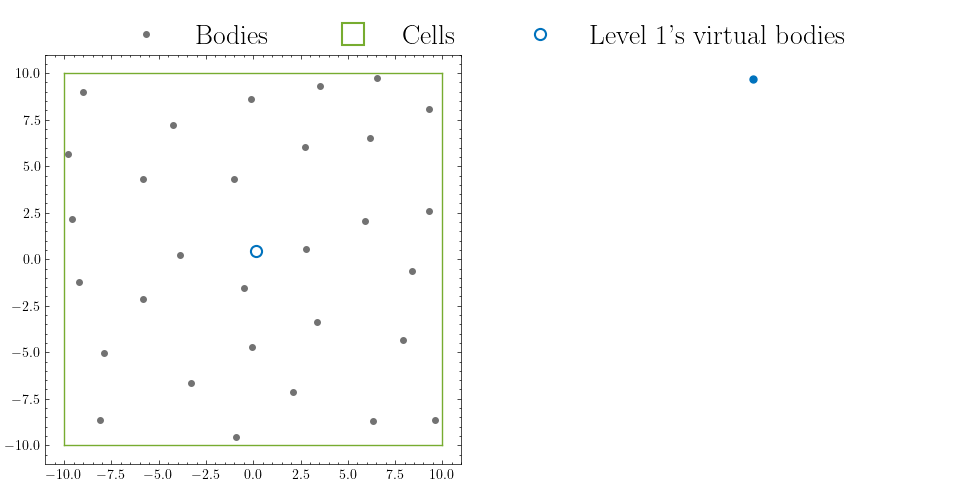
Build a root cell containing all bodies.
If a cell contains more than one body, subdivide it into 8 subcells (in 3D) at its geometric center (or center of mass).
Repeat this process recursively for each subcell until each last-stage cell contains at most one body.
For each node in the tree, compute a virtual body located at the center of mass of all bodies contained in that node, with total mass equal to the sum of their masses.

Compute Forces

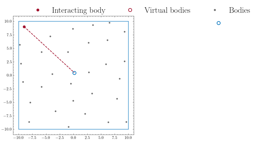
For each body, traverse the tree starting from the root.
For a given node, compute the ratio $\frac{s}{d}$ where $s$ is the size of the cell and $d$ is the distance between the body and the node's center of mass.
If $\frac{s}{d} < \theta$ ( the virtual body is far compared to its typical size):
- Approximate the interaction using the node's virtual body.
Else:
- Recursively apply the same procedure to the node's children.

Once all forces are computed, we integrate the system in time using the Verlet integrator.

The $\log N$ factor in the complexity comes from the tree traversal and recursive subdivision of space. You can see this method as a 3D analog of a dichotomy algorithm.

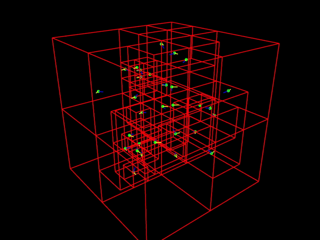
Implementation and Visualization

This algorithm is particularly well-suited for large-scale simulations and high-performance computing. It is, in fact a bit overengineered for small systems like $N = 300$ .

For this reason, the implementation was done directly in C++, using object-oriented programming for clarity. Only the force computation was parallelized, as the tree construction itself is not trivially parallelizable.

For the largest simulations ( $N = 100000$ ), we used an AWS EC2 instance with hundred CPUs.

Another challenge at this scale is visualization. I developed a small Processing-based pipeline for this purpose, but it remains relatively slow and limited. A more robust solution could be to explore visualization tools such as Blender.

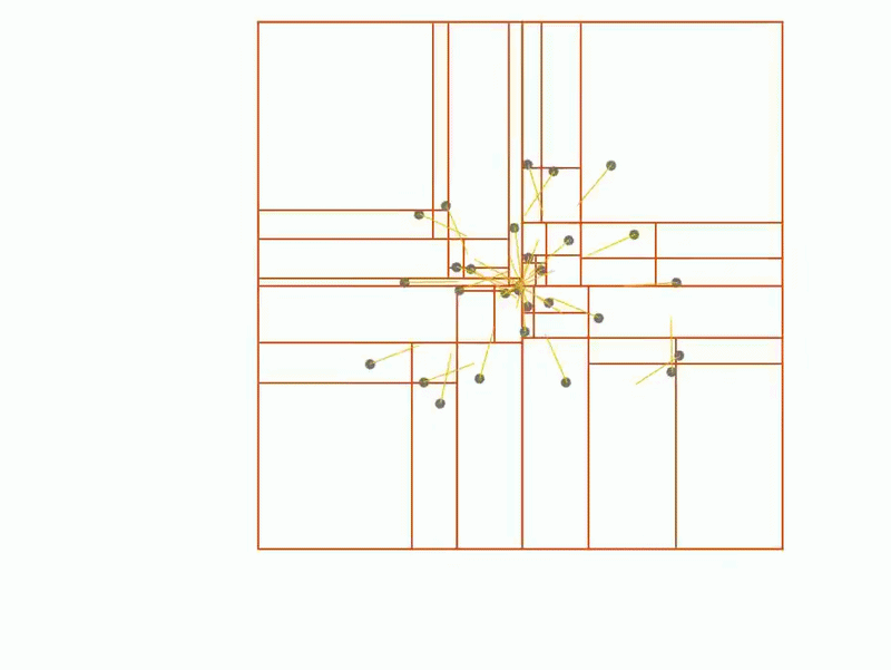
Hyperparameter, Error, and Complexity

The quality of the force calculation is entirely controlled by the hyperparameter $\theta$ . Its impact on the "resolution" of interactions can be visualized below:

Impact of θ on force calculation resolution.

As expected, decreasing $\theta$ improves accuracy, but also increases computational cost.

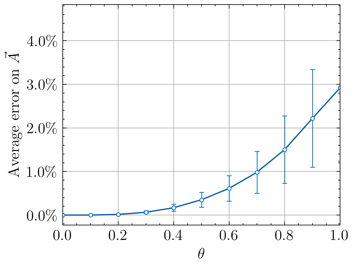
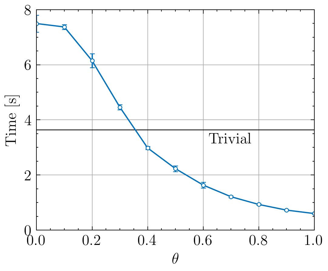
Impact of θ on one step computation time.

In practice, this trade-off is not a major issue. For large $N$ , the system becomes highly chaotic, and obtaining precise quantitative agreement is often unrealistic. Since we are mainly interested in qualitative behavior, we can choose a value of $\theta$ that provides a good balance between accuracy and performance.

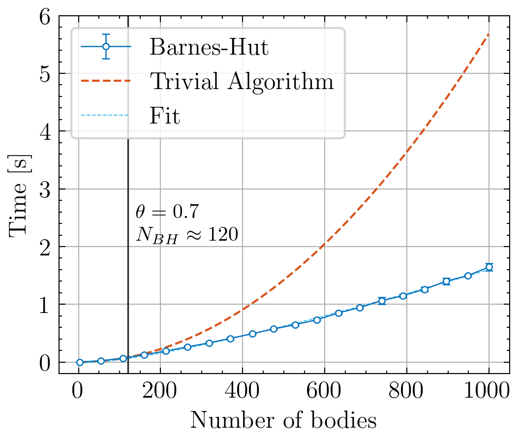
We can also compare the computational complexity of the naive approach, $O(N^2)$ , with the Barnes–Hut method, $O(N \log N)$ :

Computational complexity comparison between naive and Barnes-Hut implementation.

Results

Finally, we can blow up our AWS budget and simulate the birth of a small galaxy — the whole point of all those efforts !

To initialize the system, we randomly place bodies within a flattened ellipsoid and assign them radial velocities according to the velocity distribution of a self-gravitating system.

Here is what we obtain:

Time evolution of a N=100000 gravitational system.

Outlooks

Big Bang simulation
BIGGEEEEEER
Go to blender for visualization
Recode properly everything
Geometric center or center of mass splitting ?