A 2D Ising model using Metropolis-Hastings (rendered live in the browser). Explores phase transitions near T_c and classify phases using ML.
Ising
Introduction
Zzz... Ising... Zzz... Metropolis... Zzz... renormalization flow... Wait, no. No no NO! I wake up.. Just a nightmare. The Ising model can’t hurt me... right?
If you’ve studied physics, mathematics, or computer science, you’ve probably heard of the Ising model. It is a quite simple toy model that turns out to illustrate a surprising number of deep concepts. In this article I will talk about some experiments I made based on this model.
Live Ising Model
The model
Originally introduced as a toy model to study magnetism in materials, the Ising model consists of a lattice of interacting spins (small quantized magnetic dipoles).
Here, we focus on the simple 2D square lattice with nearest-neighbor interactions.
Mathematically, the system is defined on a periodic square lattice of size . Each site can take one of two values: (up) or (down). A configuration of the system is denoted by . The total energy is given by
where denotes summation over nearest neighbors, is the coupling constant (which we set to ), and is an external magnetic field.
Using statistical physics and the canonical ensemble, we define the partition function
which gives rise to the probability distribution over configurations:
For any observable defined on configurations, its expected value is
One of the most important observables in the Ising model is the mean magnetization:
This quantity plays a central role, as it allows us to detect a key feature of the 2D Ising model: a phase transition. At low temperature, spins tend to align, leading to a non-zero magnetization. At high temperature, thermal fluctuations dominate and the spins become disordered, so the magnetization vanishes.
Another important observable is the spin–spin correlation function, which measures how spins separated by a distance are related:
This function provides deeper insight into the structure of the system: at high temperature, correlations decay rapidly with distance, while near the critical temperature they persist over long ranges, reflecting the emergence of large-scale collective behavior.
Indeed, the 2D Ising model was solved analytically by Onsager, who showed that the system undergoes a phase transition at the critical temperature
Sampling the distribution with MCMC
Mathematically, the system defines a complex probabilistic model parameterized by the temperature (and the external magnetic field). Unfortunately, this distribution is not easy to sample from directly, or to study analytically.
A standard approach is to use Markov Chain Monte Carlo (MCMC), in particular the Metropolis–Hastings algorithm. I am too lazy to go through full derivation here, but as you know, Wikipedia is our best friend !
Algorithm
At each step:
- Select a lattice site
- Compute the energy difference if we flip that spin
- If , accept the flip
- Otherwise, accept it with probability
- Repeat
This defines a Markov chain whose stationary distribution is exactly the Boltzmann distribution .
Implementation
This simple algorithm can be implemented efficiently in Python. I represent the 2D lattice as a 1D array of boolean variables.
During this project, I also discovered a surprisingly powerful (and underrated) feature which sometimes allows near-C performance with minimal effort. Let me introduce you the holy @njit decorator from Numba !
@njit(fastmath=True)The function that performs one Metropolis step is:
@njit(fastmath=True)
def stepMetropolis(L,grid,boltzCoefs):
    ind = np.random.randint(0,L*L)
    count =  grid[ind%L + L*((ind//L+1)%L)] + grid[ind%L + L*(((ind//L)-1)%L)] + grid[(ind%L-1)%L + L*((ind//L)%L)] + grid[(ind%L+1)%L + L*((ind//L)%L)]
    if np.random.random() < boltzCoefs[count+5*grid[ind]]:
        grid[ind] = not (grid[ind])
    return grid
Here, boltzCoefs are precomputed probabilities for flipping spins, depending on the local configuration (neighboring spins and current spin value):
Thermalization and decorrelation
A crucial point when using MCMC is that samples are not independent.
Since each configuration is obtained from the previous one by a small local update, the system evolves slowly through configuration space. As a result:
- Early samples are biased by the initial condition (thermalization issue)
- Consecutive samples are strongly correlated (autocorrelation issue)
To address this:
- Thermalization: Before taking any measurement, the system must be evolved for many steps until it reaches equilibrium.
- Autocorrelation: Even after thermalization, configurations remain correlated over many steps. The number of steps required to produce an effectively independent sample is called the autocorrelation time.
Near the critical temperature , this becomes particularly bad.
In practice, there are several strategies:
- Only record one sample every steps (decorrelation time)
- (More advanced) use cluster algorithms like Wolff or Swendsen–Wang
- (Even more advanced) use ML-based methods near criticality ! I will investigate this later...
In my case, I took the simple (but costly) approach: I re-thermalize a random lattice for each sample to completly kill correlations between samples.
Some results
With this algorithm, we can generate samples at different temperatures and study their properties.
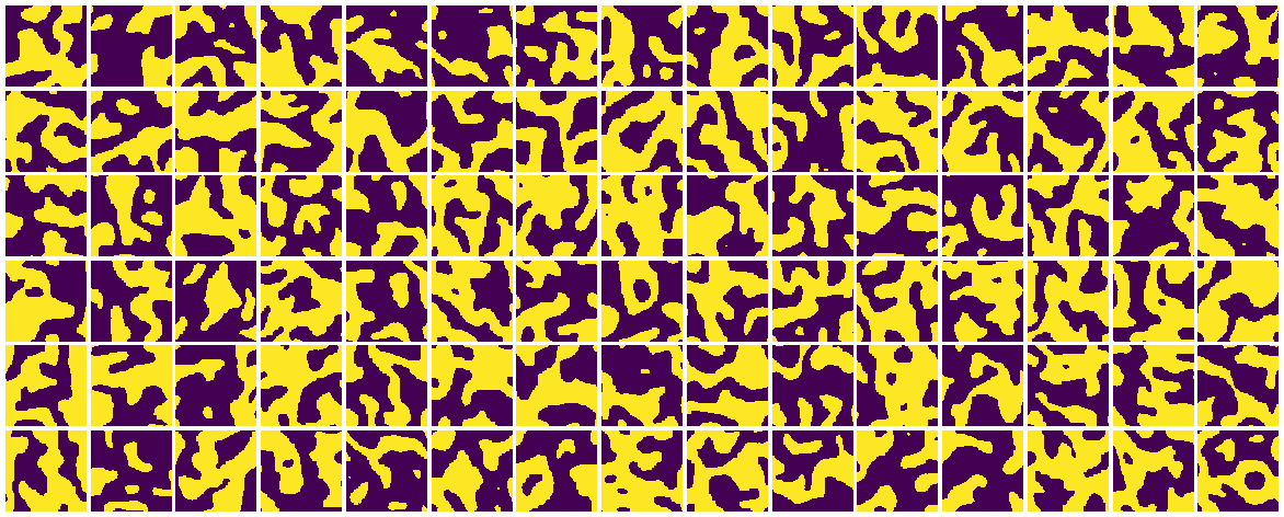
We can then compute observables such as the magnetization or spin–spin correlation:
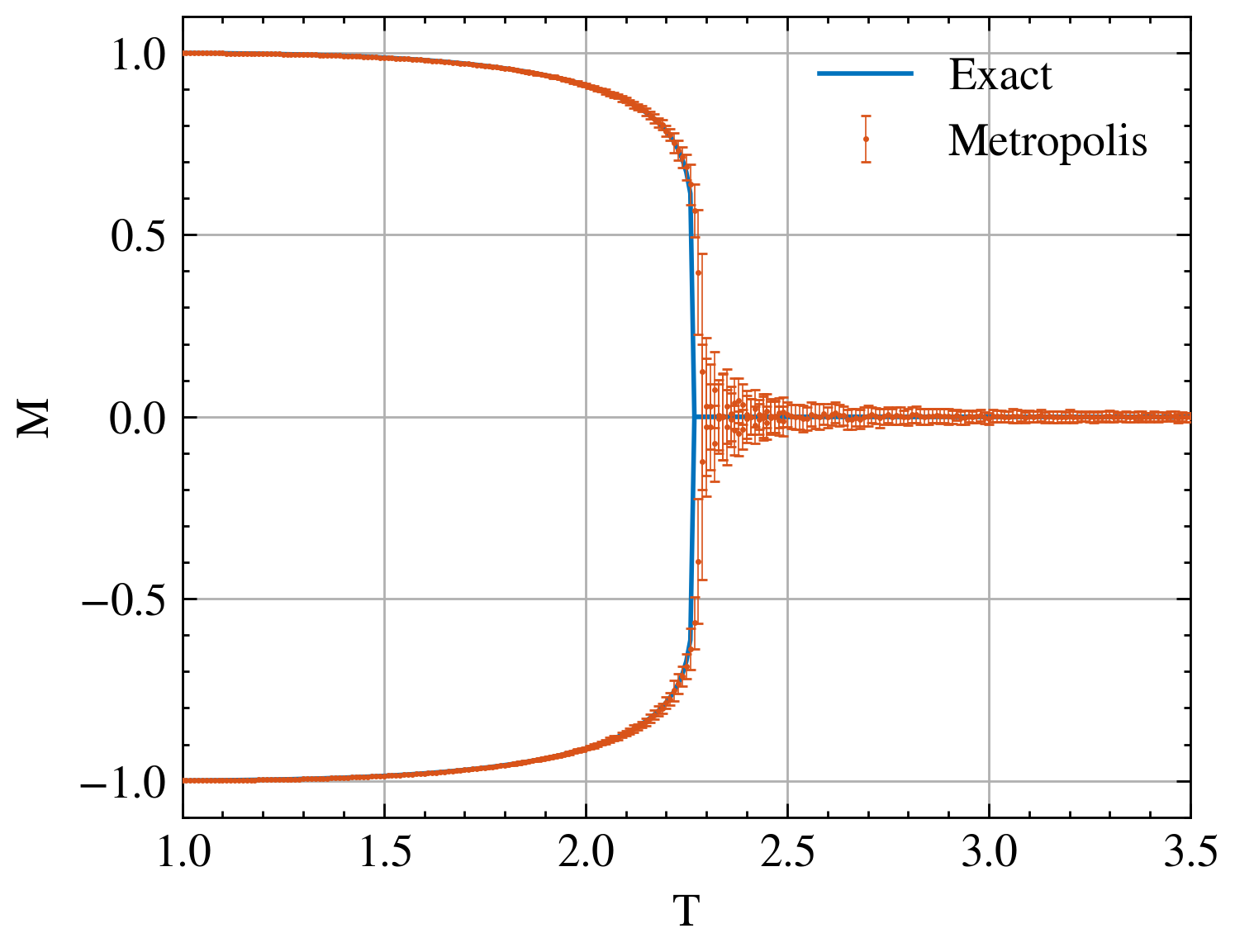
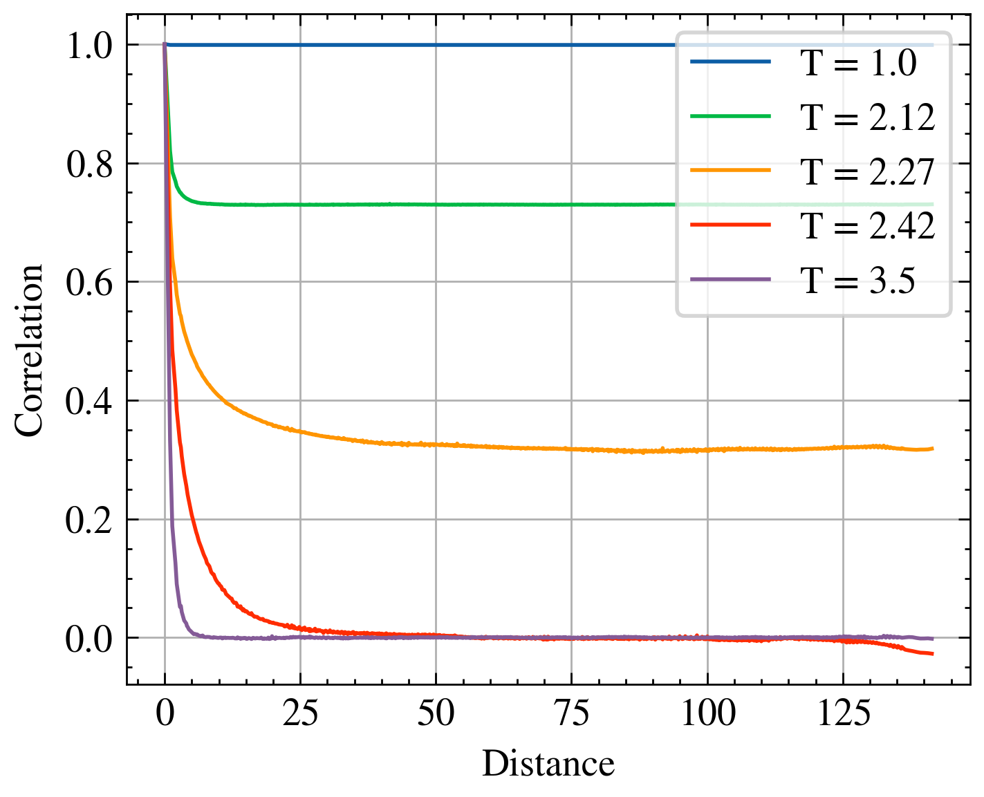
These results clearly illustrate the famous phase transition of the 2D Ising model: below a critical temperature of approximately , spins become strongly correlated and a global magnetization emerges. This behavior is directly related to the Curie temperature observed in ferromagnetic materials.
Study by renormalization
// To be written
Phase classification using CNNs
// To be written, my proof of concepts works so further results to come...
ML sampling methods
- Energy-based Models
- Diffusion Models