// numerical-physics · informatics · physics·

Mar. 2026·8 min read

Simulation of a high-voltage electric discharge in a dielectric medium. Based on an electronic field solver + a stochastic cellular automaton, the Dielectric Breakdown Model.

Tesla Coil Pt.3, Electric Discharge Simulation

Introduction

After my Tesla Coil project, I developed a strong addiction to the hypnotic patterns traced by high-voltage discharges in air. Unfortunately, my DIY Tesla coil is not very portable, and has a tendency to interfere with surrounding electronic devices (RIP my wahing machine). But what if me can simulate the discharge process ? My hunger will finally be satisfied...

Live Dielectric Breakdown

grid

SOR sweeps/frame5

cpu load0%

grid

SOR sweeps/frame5

cpu load0%

view

η branching2.5

ω SOR1.955

What is Lightning?

At its core, a lightning bolt is an ionic channel that conducts electric current through air, which is normally a dielectric (non-conductive) medium. Here is how it forms:

An electric potential difference builds up between two conductors separated by a dielectric medium, usually caused by a charge imbalance (for instance, between a storm cloud and the ground).
This spatial variation in potential generates an electric field $\vec{E} = -\nabla \phi$ , which accelerates the few free charges naturally present in the air.
Where the field is strong enough, these accelerated charges collide with air molecules with sufficient energy to strip away outer electrons, generating new free charges. This triggers a cascade, a self-sustaining avalanche, as long as the field remains strong enough.
This process propagates from one electrode to the other: electrons travel from the negative to the positive side.
Throughout the process, the electric field continuously adapts to the evolving charge distribution. Many stochastic phenomena occur along the way, giving lightning its characteristic branching, exploratory pattern.

Simulation

This simulation is based on the Dielectric Breakdown Model and has to be taken as a qualitative physically informed model. The simulation of a complete breakdown process requires much more attention and work.

We model this on a 2D lattice with two objects: an electric potential field $\phi$ , and a boolean mask representing the ionic channel. At each time step, the simulation alternates between two operations:

Solve the electric field on the lattice
Advance the ionic channel by one cell, using a probability distribution derived from the field strength

Solving the Field

The ionic channel is a conductor, so it imposes an equipotential boundary condition on the field. Since this boundary changes at every step, one new cell joins the channel each time, the field must be recomputed after each step. Fortunately, because only one cell changes per step, the field evolves slowly and we can warm-start the solver from the previous solution, which makes iterative methods very efficient here.

The field satisfies the Laplace equation outside of fixed potential site (electrodes and ionic channel).

\nabla^2 \phi = 0

On a 2D lattice, the Laplacian can be discretised using a 5-point or 9-point finite difference stencil:

\begin{aligned} \nabla^2 \phi_{i,j} \approx \frac{1}{\Delta x^2}\left(\phi_{i+1,j}+\phi_{i-1,j}+\phi_{i,j+1}+\phi_{i,j-1}-4\phi_{i,j}\right) \end{aligned}

\begin{aligned} \nabla^2 \phi_{i,j} &\approx \frac{1}{6\Delta x^2}\Big[4\left(\phi_{i+1,j}+\phi_{i-1,j}+\phi_{i,j+1}+\phi_{i,j-1}\right)\\ &\qquad+\left(\phi_{i+1,j+1}+\phi_{i-1,j+1}+\phi_{i+1,j-1}+\phi_{i-1,j-1}\right)-20\phi_{i,j}\Big] \end{aligned}

The 9-point stencil includes diagonal neighbours and is isotropic, meaning it treats all directions equally, which turns out to significantly accelerate convergence, as shown below.

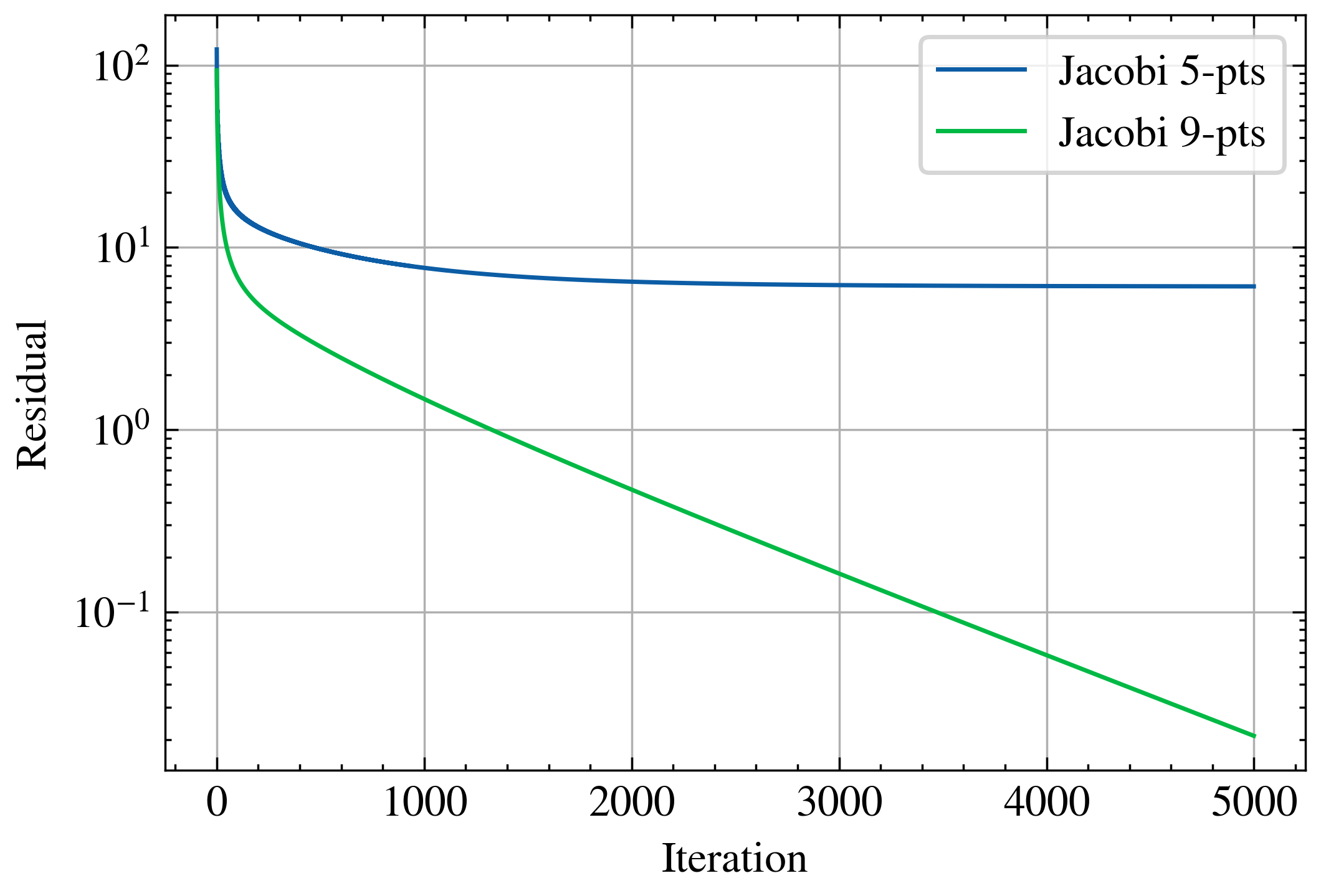
We will use the 9-point stencil throughout. Three iterative solvers of increasing sophistication are considered.

Jacobi

The simplest approach: update every cell using only values from the previous iteration.

phi_new[i, j] = ( phi[i+1, j] + phi[i-1, j] 
                + phi[i, j+1] + phi[i, j-1] ) / 5. +
                ( phi[i+1, j+1] + phi[i-1, j+1] 
                + phi[i-1, j-1] + phi[i+1, j-1] ) / 20.

Gauss-Seidel (GS)

Essentially the same as Jacobi, but each cell is updated in-place immediately, so neighbouring cells already updated in the current sweep are reused. This typically converges about twice as fast.

phi[i, j] = ( phi[i+1, j] + phi[i-1, j] 
                + phi[i, j+1] + phi[i, j-1] ) / 5. +
                ( phi[i+1, j+1] + phi[i-1, j+1] 
                + phi[i-1, j-1] + phi[i+1, j-1] ) / 20.

Successive Over-Relaxation (SOR)

SOR extends Gauss-Seidel by introducing a relaxation factor $\omega \in (1, 2)$ , which over-shoots each update to accelerate convergence. For an optimal choice of $\omega$ , convergence can be dramatically faster than plain Gauss-Seidel.

phi[i, j] = (1-omega) * phi[i, j] +
            + omega * (
                ( phi[i+1, j] + phi[i-1, j] 
                + phi[i, j+1] + phi[i, j-1] ) / 5. +
                ( phi[i+1, j+1] + phi[i-1, j+1] 
                + phi[i-1, j-1] + phi[i+1, j-1] ) / 20.
            )

The theoretical optimum for a regular domain is:

\omega_{th} = \frac{2}{1+\sqrt{1-\rho^2}} \quad \text{with} \quad \rho = \frac{\cos(\pi / N_x) + \cos(\pi / N_y)}{2}

Sweep Direction

Both GS and SOR update cells sequentially, so the order in which cells are visited matters. A fixed sweep direction (row by row, left to right) breaks isotropy: information propagates faster along the sweep direction than against it, introducing a subtle directional bias in the field. Using a random sweep direction (over 8 possibilities) at each iteration restores isotropy at the cost of some efficiency.

Picking cells at random (rather than in a sweep) kills convergence entirely, as it destroys the propagation mechanism that makes these algorithms fast(experimentally checked).

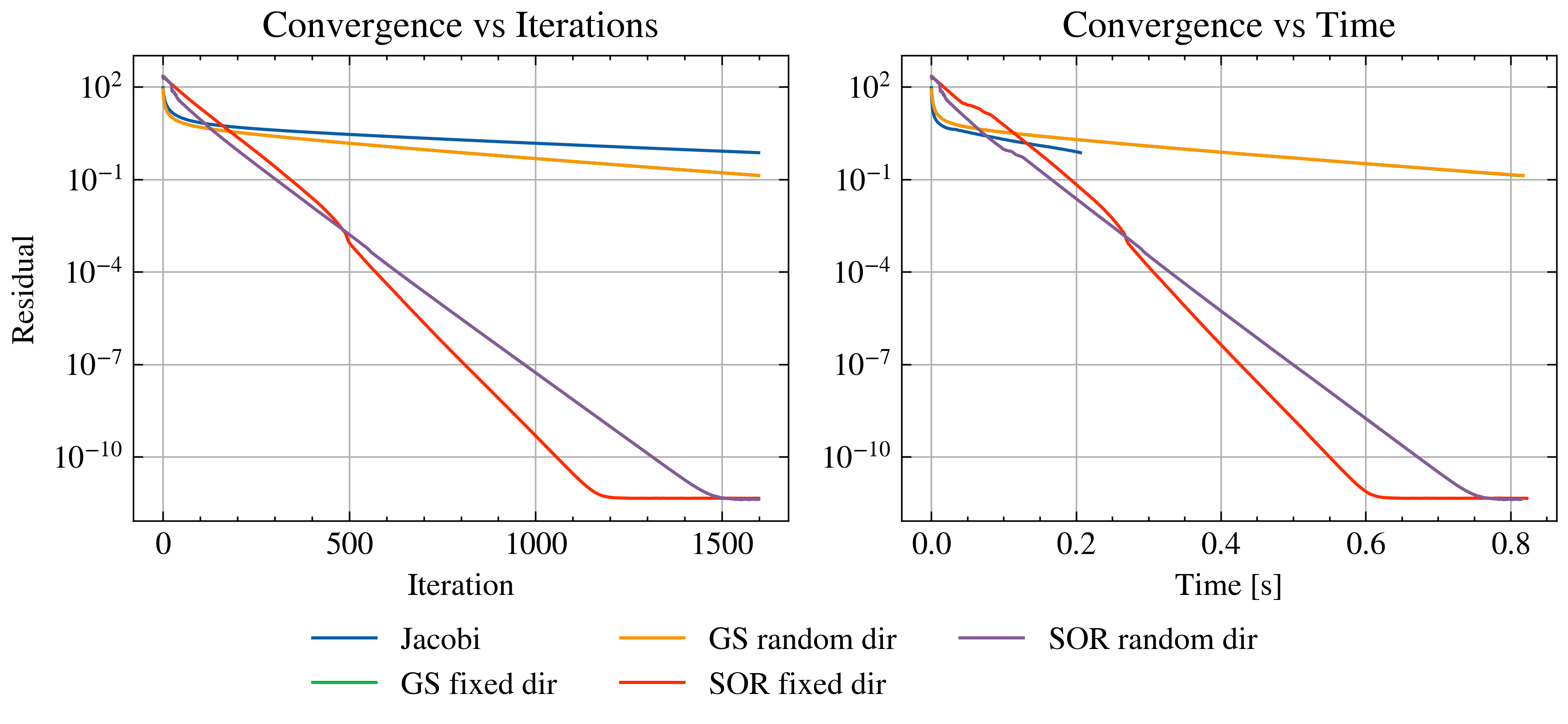
Convergence comparison between Jacobi, Gauss-Seidel, and SOR.

SOR clearly outperforms the others. It does require tuning $\omega$ , so we verify how close the theoretical optimum is in practice:

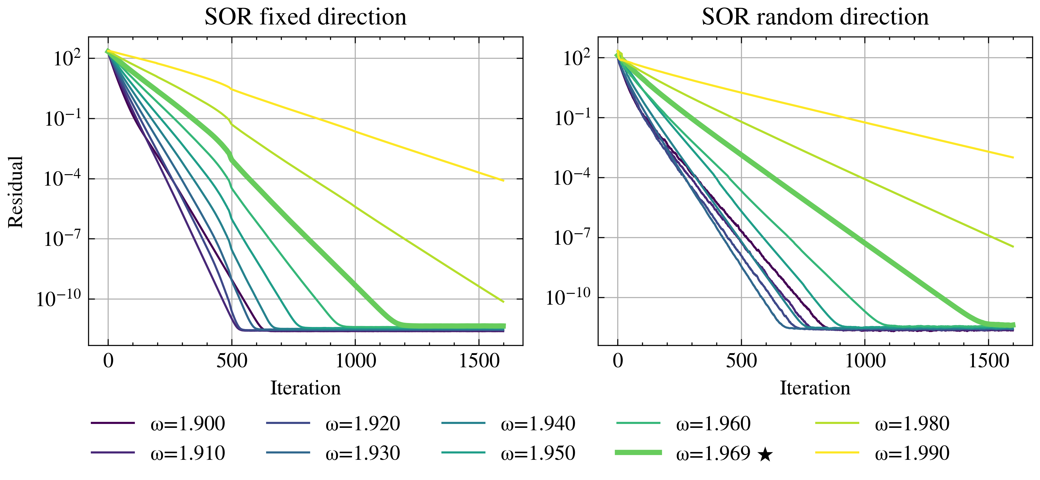
SOR convergence for various $\omega$ values around the theoretical optimum, with fixed and random sweep directions. With $\omega_{th} = 1.969$.

The theoretical value is close to the empirical optimum, though performance varies noticeably in between (up to ~50% difference). Since high precision is not required here, we use the theoretical $\omega$ with a random sweep direction.

Advancing the Channel

Now we need to determine where the ionization happen through a stochastic process. At each step, we consider all cells neighbouring the current ionic channel (including diagonals) as candidates for the next breakdown site. A cell bordering the channel at multiple points is physically more likely to break down, so each candidate is weighted by $\alpha(x)$ , the number of channel cells adjacent to it, with diagonal neighbours down-weighted by $1/\sqrt{2}$ .

For each candidate, the local field strength is estimated via the symmetric finite difference gradient:

|\vec{E}(x_i)| \approx \frac{1}{2\Delta x}\sqrt{\left(\phi(x_{i+1}) - \phi(x_{i-1})\right)^2 + \left(\phi(x_{j+1}) - \phi(x_{j-1})\right)^2}

The next cell to join the channel is then sampled from the probability distribution:

P(x) \propto \alpha(x)\, |\vec{E}(x)|^\eta

The exponent $\eta$ controls the branching behaviour. A high $\eta$ amplifies differences in field strength, making the strongest candidate overwhelmingly likely to win — the channel grows sharp and directed. A low $\eta$ flattens the distribution, giving weaker candidates a real chance, which produces diffuse, highly branched structures closer to real lightning.

Results

Field convergence with randomised sweep direction (with a speedup for visualisation).

Field convergence with a fixed sweep direction (with a speedup for visualisation).

Dielectric discharge with the electric field and its field lines.

Ten dielectric discharges, with a luminous halo for a photorealistic rendering.

These cool results qualitatively reproduced the pattern made by lightning! They also clearly illustrate the point effect (high electric field on pointy objects) that is exploited in lightning rods. In fact, we see that most of the lightning strikes on the spike. We can even observe small corona discharge from the electrodes, where tiny ionic channels build in parallel with the main one.