// numerical-physics · informatics · physics·

July 2020·8 min read

Multi-physics simulation of my Tesla Coil. The inductance and coupling of coils ate calculated, and used with a time-domain electronic solver.

Tesla Coil Pt.2, Simulation

Introduction

For my previous Tesla Coil project, I wanted to better understand the physical principles behind the machine, and to experiment with the effect of geometry and component choices on its behaviour.

In this artical, concise and technical, I study the inductive coupling between coil geometries, then use this data to build a real-time electronic simulation of the full Tesla Coil cycle.

The Inductance and Magnetic coupling

Parametrization

A general coil geometry can be described by the following parametrization, where $t \in [0, 1]$ :

\bm{r}(t) = \left( \begin{align*} ((1-t)r +& tR) \cos(2\pi N_\text{turn} t) \\ ((1-t)r +& tR) \sin(2\pi N_\text{turn} t) \\ &L(t - 0.5) \end{align*}\right) + \text{rotation} + \text{translation}

This allows for a conical coil (when $r \neq R$ ) that reduces to a standard cylindrical coil when $r = R$ . The parameter $N_\text{turn}$ controls the number of turns and $L$ the total length of the coil.

In the case of my DIY Tesla Coil, the system is modelled with the following parameters, where coil 1 is the primary and coil 2 is the secondary:

r1 = 0.1            r2 = 0.05
R1 = 0.25           R2 = 0.05
n1 = 9              n2 = 1200
L1 = 0              L2 = 2*w2*n2 = 0.4
w1 = 0.01           w2 = 0.000165
z01 = 0.02          z01 = 0.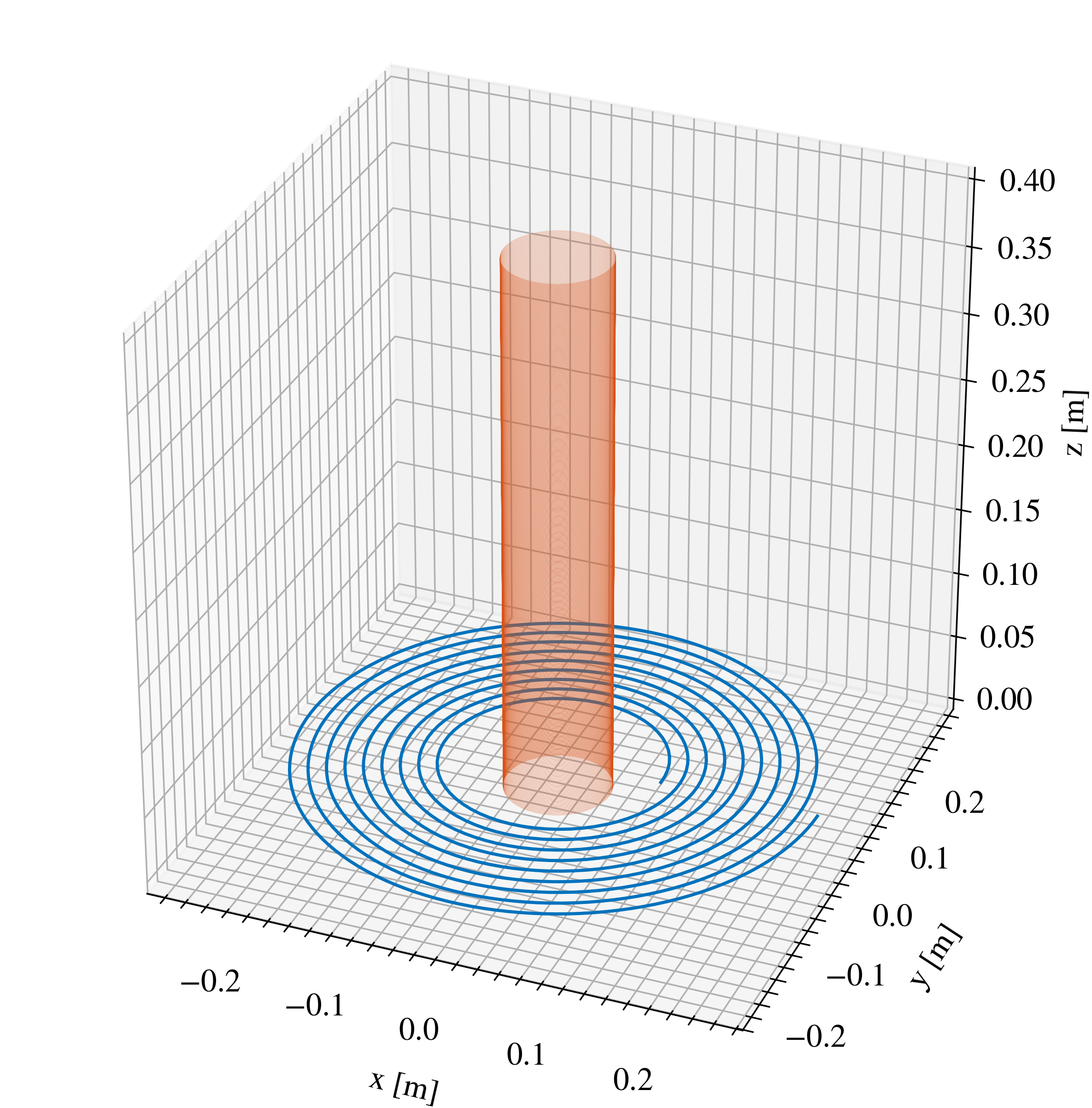

The two coils under study (blue: primary, orange: secondary).

It is useful to reparametrize the curve with an arc-length parametrization, one where the "speed" $|d\bm{r}/dt|$ is constant. This ensures that when the curve is discretized numerically, all segments have the same length, which may be important for the accuracy of finite element methods.

The arc length as a function of $t$ is:

s(t) = \int_0^t \left| \frac{d\bm{r}}{dt'}(t') \right| dt'

If we can express $t(s)$ , then $\bm{r}(t(s))$ is arc-length parametrized. While $s(t)$ can in principle be computed analytically for our coil, the expression is complicated and cannot be inverted in closed form. We therefore compute the reparametrization numerically:

def equinorm_integral(f):
    """Compute cumulative arc length along a discretized curve f of shape (N, 3)."""
    d_dist = np.sqrt(np.diff(f[..., 0])**2 +
                     np.diff(f[..., 1])**2 +
                     np.diff(f[..., 2])**2)
    return np.concatenate(([0.], np.cumsum(d_dist)))
 
def equinorm_param(t, f):
    """Return values of t that produce uniformly spaced arc-length samples."""
    s_of_t = equinorm_integral(f)
    s_of_t /= s_of_t[-1]
 
    t_of_s = interp1d(s_of_t, t, axis=0)
    s_uniform = np.linspace(0, 1, len(t))
    return t_of_s(s_uniform)

Physical model

A coil is electrically described by its self-inductance $L_i$ and its coupling $k_{ij}$ to other coils. This coupling arises from the variation of magnetic fields generated by other coils. Concretely, the voltage across coil $i$ is:

V_i = L_i\frac{dI_i}{dt} + \sum_j M_{ij}\frac{dI_j}{dt}

where the coupling depends on the mutual inductance through:

k_{ij} = \frac{ M_{ij} }{ \sqrt{L_i L_j} }

The mutual inductance between two coils $i$ and $j$ can be calculated using the Neumann formula:

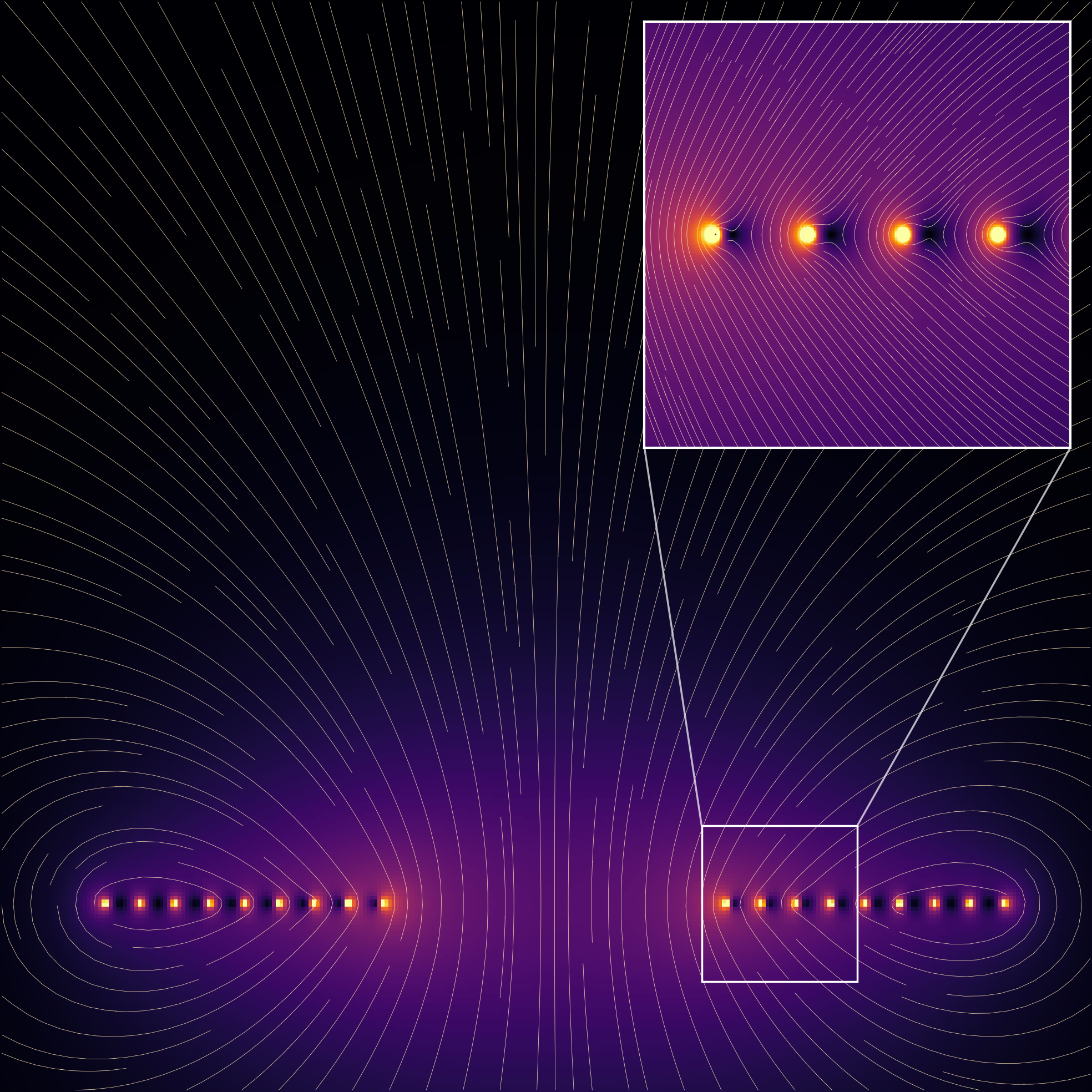
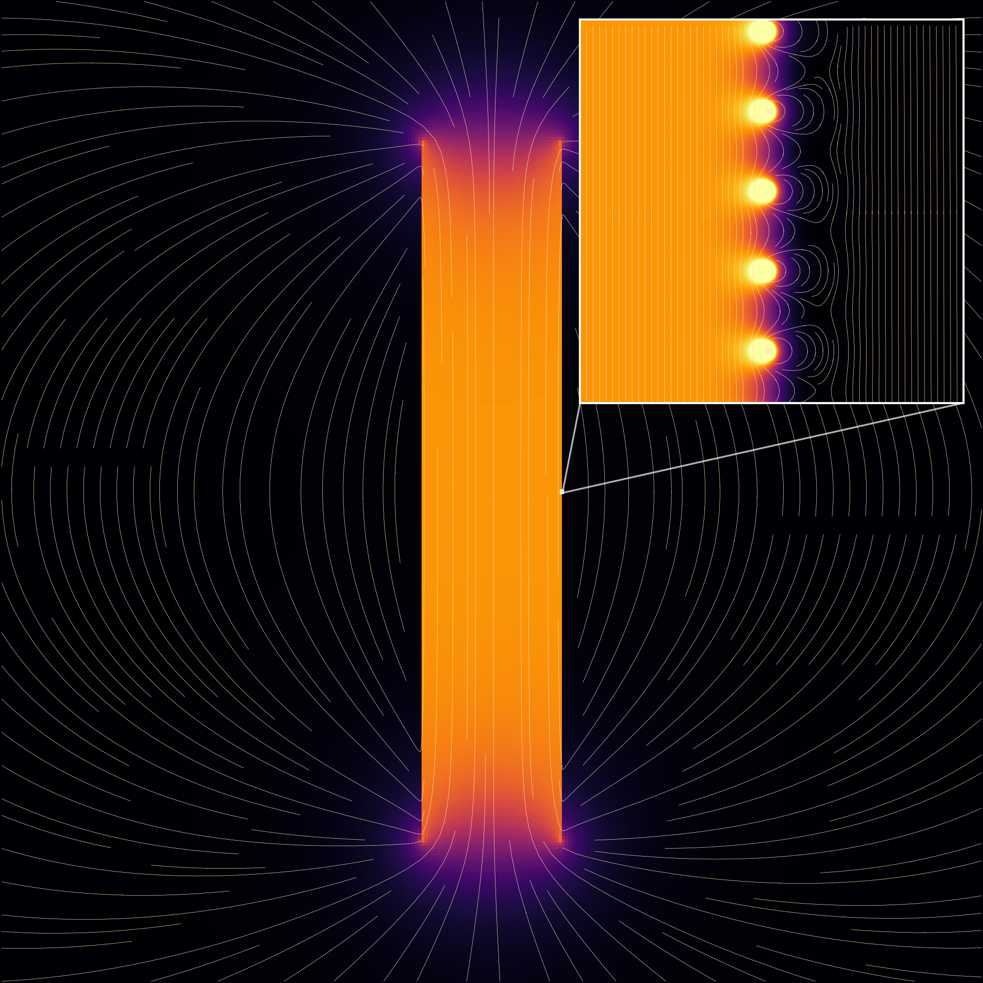
M_{ij} =\frac{\mu_0}{4\pi} \int_{C_i}\int_{C_j} \frac{ d\bm{l}_1 \cdot d\bm{l}_2 }{|\bm{r}_1 - \bm{r}_2|}

The magnetic field generated by a coil is given by the Biot–Savart law:

\bm{B}(\bm{r}) = \frac{\mu_0 I}{4\pi} \int_{C} d\bm{r'} \times \frac{ \bm{r} - \bm{r'}}{|\bm{r} - \bm{r'}|^3}

Magnetic field

We model each coil as a series of straight segments, where each segment is located at $\bm{r_0}$ , oriented along unit vector $\bm{u_0}$ , and has length $\ell_0$ . The exact magnetic field generated by a single such segment is:

\begin{align*} \bm{B}(\bm{r}) & = \frac{\mu_0 I}{4\pi \gamma} \left( \frac{\ell_0 + \beta }{ \sqrt{(\ell_0 + \beta)^2 + \gamma}} - \frac{ \beta }{ \sqrt{\beta^2 + \gamma}} \right) \bm{u_0} \times (\bm{r} - \bm{r_0}) \\ \text{ with } & \beta = \bm{u_0} \cdot (\bm{r} - \bm{r_0})\\ \text{ and } & \gamma = |\bm{r} - \bm{r_0}|^2 - \beta^2 \end{align*}

The total field of the coil is then obtained by summing the contributions of all segments, this is essentially a finite element approach.

Coupling

Deriving an exact closed-form solution for the mutual inductance integral between two arbitrary coils is generally intractable. We therefore approximate the Neumann double integral as a double sum over segment midpoints $\bm{x}_i$ , where $\bm{\Delta x}_i$ is the vector representing each segment (encoding both direction and length):

M_{ij} = \frac{\mu_0}{4\pi}\sum_{\bm{x}_i} \sum_{\bm{x}_j} \frac{ \bm{\Delta x}_i \cdot \bm{\Delta x}_j }{|\bm{x}_i - \bm{x}_j|}

Analytical induction and coupling

For validation, we can also use a theoretical result for the mutual inductance of two coaxial loops of radii $R_i$ , $R_j$ separated by a distance $d$ :

\begin{align*} m_{ij} &= \mu_0\sqrt{R_i R_j} \frac{2}{k} \left( \left(1-\frac{k^2}{2}\right)K(k^2) - E(k^2) \right)\\ \text{ with }& k^2 = \frac{4 R_i R_j }{ (R_i + R_j)^2 + d_{ij}^2} \end{align*}

where $K$ and $E$ are the complete elliptic integrals of the first and second kind, respectively.

The self-inductance of a single loop of radius $R$ with wire radius $\rho$ is:

\ell_{i} = \mu_0 R \left( \log \left( \frac{8R}{\rho} \right) - 2 \right)

From these two results, the total self-inductance of a coil (summing each loop's self-inductance and all mutual interactions between loops) and the total mutual inductance between two coils can be reconstructed by summing the appropriate $\ell_i$ and $m_{ij}$ terms.

When the winding density is high (many turns per unit length), the coil can be modelled as a continuous cylindrical sheet of conductor. In this limit, the self-inductance becomes:

L \approx \frac{\mu_0 \pi N^2 R^2}{L_c} \cdot \frac{L_c}{L_c+0.9R}

where $N$ is the number of turns, $R$ is the coil radius, and $L_c$ is the physical length of the coil. The factor $\frac{L_c}{L_c+0.9R}$ is the Nagaoka correction, which accounts for the finite length of the coil (this is itself an approximation of the exact Nagaoka function).

Results

For the studied coil configuration, we obtain the magnetic field and the self and mutual inductance.

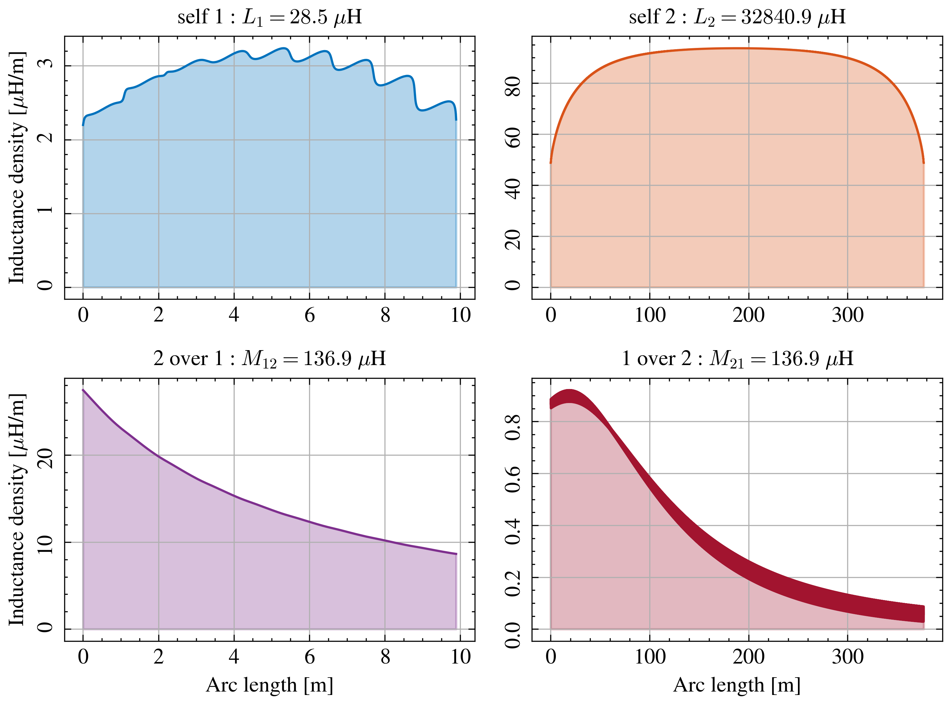
Self and mutual inductance between coil 1 and 2, along their length.

    === COIL 1 ===
Length = 9.8972 m
R = 0.0005 Omhs
L (analytic)     = 28.1104 μH
L (simulation)   = 28.4587 μH
 
    === COIL 2 ===
Length = 376.9913 m
R = 74.0496 Omhs
L (analytic)            = 31950.6411 μH
L (analytic continuous) = 31937.5963 μH
L (simulation).         = 32840.9457 μH
 
    === COUPLING ===
M (analytic)    = 139.8130 μH -> k = 0.1475
M (simulation)  = 136.9115 μH -> k = 0.1416

These numerical results can be used as parameters in my circuit simulation of my Tesla Coil.

Electronic part

// to be written

Tesla Coil pt.1, DIY

Design and building of a Tesla coil capable of producing 30cm arcs. It is based on two RLC resonnant circuits.

// diy · physics